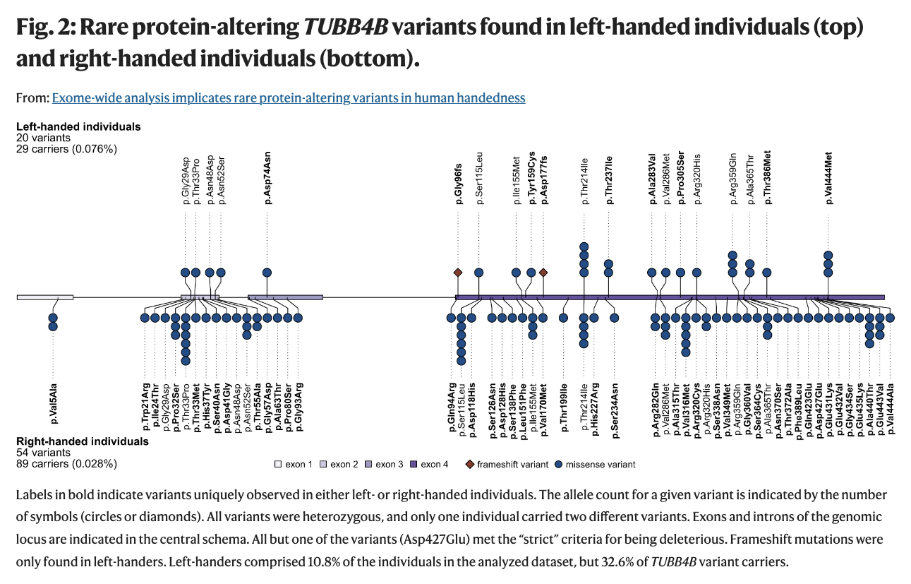
Are you a lefty? Well, I am. And so was my mom. And her father. AND our daughter. So I was curious to learn how rare genetic factors may contribute to the roughly 10% of us who are left-handed. As reported in GenomeWeb, researchers at the Max Planck Institute for Psycholinguistics in the Netherlands and Radboud University used exome data from the UK Biobank to search for clues. What they found is that variations in the beta-tubulin gene TUBB4B occurred at a rate 2.7 times higher in left-handers than right-handers.
TL;DR I did not find these rare variants, but it never hurts to look.
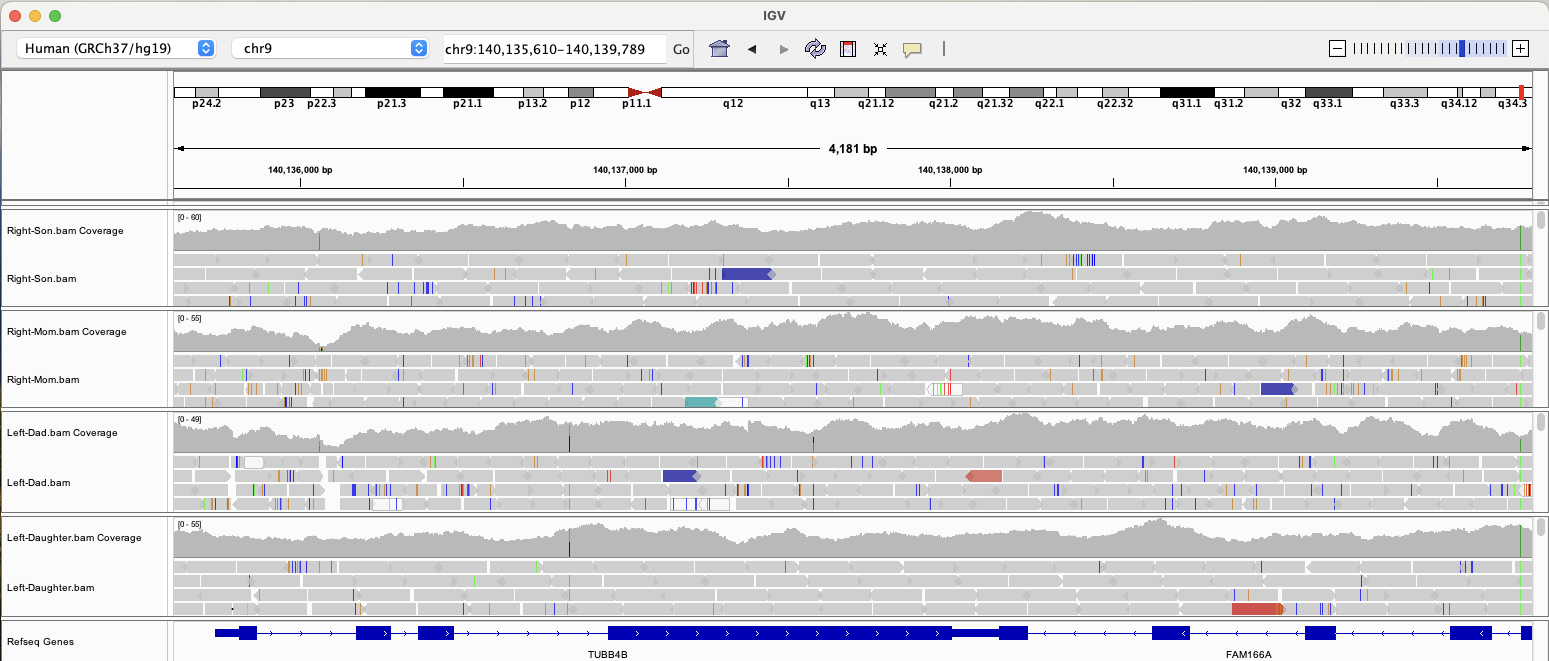
Naturally, I wanted to see if our daughter and I shared any of these mutations, so I fired up IGV to visualize our WGS data and take a look at TUBB4B. (Click the image to make it larger.)
It turns out that we do not have any of the rare mutations mentioned in the paper, but then again, these particular variations explain only 0.91% of expected heritability. (Left-handedness shows heritability of ~25% in twin-based analysis.)
In August 2021, I joined Amazon Web Services (AWS) as an industry specialist, completing a personal, 12-year goal to work in precision medicine. At AWS, I work with leading-edge customers in areas such as cancer detection, disease diagnostics, clinical trials, population health, and drug discovery. All the cool stuff!
In our spare time, we wrote a paper to investigate how mRNA, microRNA, and protein expression levels change as kidney cancer patients progress to different disease stages.
Here’s the preprint abstract on medRxiv (Nov 2022):
Renal clear cell carcinoma (RCC), the most common type of kidney cancer, lacks a well-defined collection of biomarkers for tracking disease progression. Although complementary diagnostic and prognostic RCC biomarkers may be beneficial for guiding therapeutic selection and informing clinical outcomes, patients currently have a poor prognosis due to limited early detection. Without a priori biomarker knowledge or histopathology information, we used machine learning (ML) techniques to investigate how mRNA, microRNA, and protein expression levels change as a patient progresses to different stages of RCC. The novel combination of big data with ML enables researchers to generate hypothesis-free models in a fraction of the time used in traditional clinical trials. Ranked genes that are most predictive of survival and disease progression can be used for target discovery and downstream analysis in precision medicine. We extracted clinical information for normal and RCC patients along with their related expression profiles in RCC tissues from three publicly-available datasets: 1. The Cancer Genome Atlas (TCGA), 2. Genotype-Tissue Expression (GTEx) project, 3. Clinical Proteomic Tumor Analysis Consortium (CPTAC).
The code for this study is available on GitHub, and we are actively submitting the paper for peer review.
After creating FASTQ files from my BAM data and learning how to use Terra, I was finally ready to run the Whole Genome Analysis Pipeline. This collection of workflows, called a “workspace,” contains the latest GATK Best Practices workflows for whole genome sequence (WGS) data, including pre-processing, germline short variant discovery, and joint variant calling. Although I am working with a single human genome (my own), this same production pipeline is routinely used on thousands of WGS samples every day.
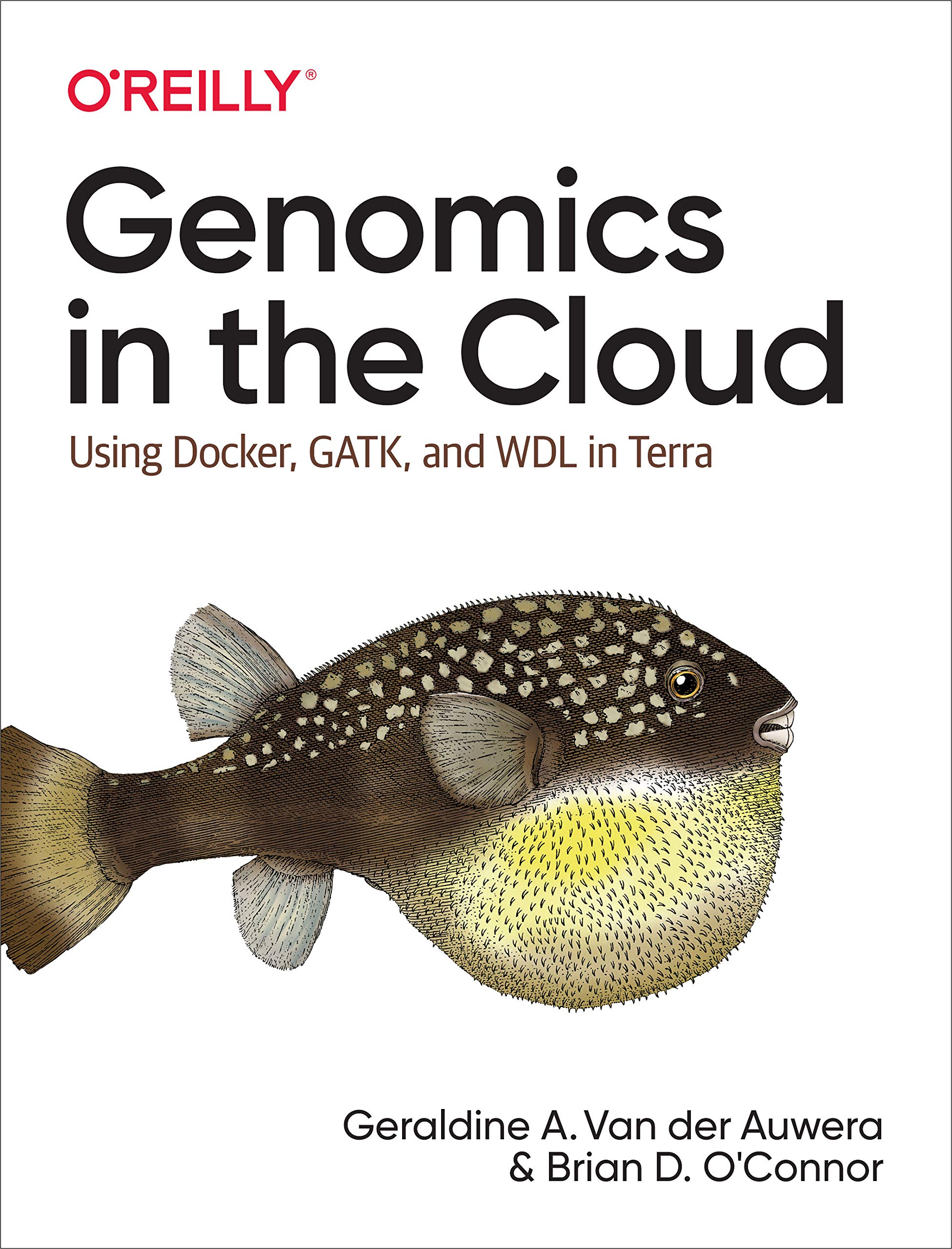
Being a relative newcomer to GATK and a complete notice with Terra, the path to success was a little bumpy. Before jumping into what I learned, I want to acknowledge the staff at the Broad, who were extraordinarily kind. Starting with with GATK’s Benevolent Dictator for Life, Geraldine Van der Auwera, who is coincidentally the co-author of a highly informative book, Genomics in the Cloud. This blog post would not be possible without the knowledge that I gleaned from those pages. The Terra support team has also been wonderfully responsive–I even received a call from a designer at the Broad asking how they could improve Terra’s user experience!
Below, I describe the reprocessing of my WGS data. The goal is to have a consistent baseline as we continue to search for answers in our genes.
Note: Terra is evolving rapidly, and you may find that some links have changed. These tips were current as of this writing (June 2021). Drop me a line on Twitter if you see an improvement that I can add.
1. Creating unmapped BAM (uBAM) files from paired end files
Our family’s WGS data was processed on Illumina sequencers, albeit on different machines at different times. To get started, the first processing step is to create unmapped BAM (uBAM) files from raw FASTQ data. GATK’s use of uBAM files is an acknowledged “off label” use of the BAM file format, but it provides an opportunity to insert details (metadata) that would otherwise be absent. Given Illumina’s 75% market share, chances are high that you will be creating uBAM files using the “Paired FASTQ to unmapped BAM” workflow located in the Sequence-Format-Conversion workspace (or something similar).
2. Read Groups (@RG) in the uBAM file
After creating uBAM files, my first run of the 1-WholeGenomeGermlineSingleSample workflow ended with an error (after three days of processing):
Task UnmappedBamToAlignedBam.CheckContamination:NA:1 failed. Job exit code 255. Check gs://my-terra-bucket/.../call-CheckContamination/stderr for more information. PAPI error code 9. Please check the log file for more details: gs://my-terra-bucket/.../call-CheckContamination/CheckContamination.log.
To start debugging the CheckContamination subtask, I fired up the cloud-based Jupyter notebook within Terra (very cool), attempted to copy the sorted BAM file to the notebook environment, and promptly ran out of disk space. To create enough disk space for your BAM file, go to settings (look for the big gear in upper right corner) and change the persistent disk size to 100 GB.
The cause of this error turned out to be a misunderstanding about read groups. In the BAM file, you can see two different values in the read group (@RG) field: Pickard-K-Thomas_C and Pickard-K-Thomas_A. Those values have to be the same; otherwise, CheckContamination thinks your BAM file has been “contaminated” with multiple samples.
The fix was to go back to Sequence-Format-Conversion and change three values in WORKFLOWS>INPUTS, which in turn inserts the correct metadata in your uBAM files–many thanks to Geraldine for pointing this out:
Change readgroup_name from this.read_group to this.read_group_id
Change sample_name from this.sample_id to this.sample
Change additional_disk_space_gb to 100
Other notes:
This article was invaluable to understand how read groups (@RG) work.
ID (Read Group IDentifier) field: Each ID value must be unique.
SM (SaMple) field: Unlike ID, the sample name must be the same in all SM fields.
LB (LiBrary) field: I referenced my unique Illumina ID for DNA prep library traceability.
PL (PLatform) = ILLUMINA (all caps)…I read an official list of sequencers in the documentation and “ILLUMINA” is on that list.
PU (Platform Unit) field: The convention is to use periods as the delimiter in the lane identifier, not underbars as used in the FASTQ filename.
CN (Sequencing CeNter) field: I used “Illumina” because they processed this sample.
DT (DaTe) field: Using the ISO 8610 combined date/time standard worked for me. Interestingly, Terra converted my local time to UTC time inside the BAM file (which makes sense given that genomes can be processed across multiple timezones).
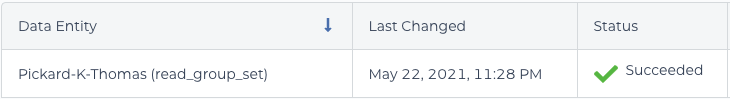
From the Sequence-Format-Conversion workflow, here’s my successful DATA>TABLE>read_group page in tsv format:
Creating uBAM files took about four hours at a cost of $1.15. It was time for a second run of the 1-WholeGenomeGermlineSingleSample workflow.
3. CheckFingerprint issue #1
This time, the sticking point was at the end of the pipeline in a routine called CheckFingerprint, which is called as a subtask within AggregatedBamQC. Here’s the error (also found after three days of processing):
Job AggregatedBamQC.CheckFingerprint:NA:1 exited with return code 1 which has not been declared as a valid return code. See 'continueOnReturnCode' runtime attribute for more details.
I checked the CheckFingerprint.log and suspected the issue was related to the NA12878 dataset (what was that doing there???):
WARNING 2021-05-11 21:25:40 FingerprintChecker Couldn't find index for file /cromwell_root/dsde-data-na12878-public/NA12878.hg38.reference.fingerprint.vcf going to read through it all.
WARNING 2021-05-11 21:25:40 FingerprintChecker There was a genotyping error in File: file:///cromwell_root/dsde-data-na12878-public/NA12878.hg38.reference.fingerprint.vcf
Cannot find sample 1-WholeGenomeGermlineSingleSample_2021-05-09T05-11-16 in provided file.
The fix for CheckFingerprint issue #1
After some head scratching, I found the solution by scrolling to the bottom of WORKFLOWS>INPUTS. There, I found a field called fingerprint_genotypes_file, which had a value of: gs://dsde-data-na12878-public/NA12878.hg38.reference.fingerprint.vcf
Note: When debugging your problem, keep in mind that searching the Terra knowledge base does not include results from GATK documentation, which can be very useful for GATK- or Picard-related issues.
4. CheckFingerprint issue #2
The third run was also unsuccessful–this time the issue was a little trickier. Here’s the error message (also found after three days of processing!):
INFO 2021-05-11 21:27:00 CheckFingerprint Read Group: null / Pickard-K-Thomas vs. 1-WholeGenomeGermlineSingleSample_2021-05-09T05-11-16: LOD = 0.0
ERROR 2021-05-11 21:27:00 CheckFingerprint No non-zero results found. This is likely an error. Probable cause: EXPECTED_SAMPLE (if provided) or the sample name from INPUT (if EXPECTED_SAMPLE isn't provided) isn't a sample in GENOTYPES file.
The fix for CheckFingerprint issue #2
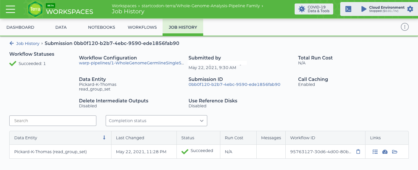
It turns out that the saved name of your WORKFLOWS>root entity>read_group_setmust match the name of your VCF output (in my case, Pickard-K-Thomas). In the error message above, the default read_group_set name (1-WholeGenomeGermlineSingleSample_2021-05-09T05-11-16) does not match, but is stored as the value in read_group_set_id in DATA>read_group_set . Saving the read_group_set name as “Pickard-K-Thomas” fixed the issue. The alternative is to change the value of WORKFLOWS>INPUTS>sample_and_unmapped_bams, which uses read_group_set_id by default. Yikes!
Note: Understanding the standard data model is critical to your success. This article, chapters 11 and 13 in Genomics in the Cloud, and these videos will assist in wrapping your head around it. I found the data model to be the most challenging part of this process.
I launched 1-WholeGenomeGermlineSingleSample for the fourth time, but aborted it after four days of processing (thinking that the software was broken).
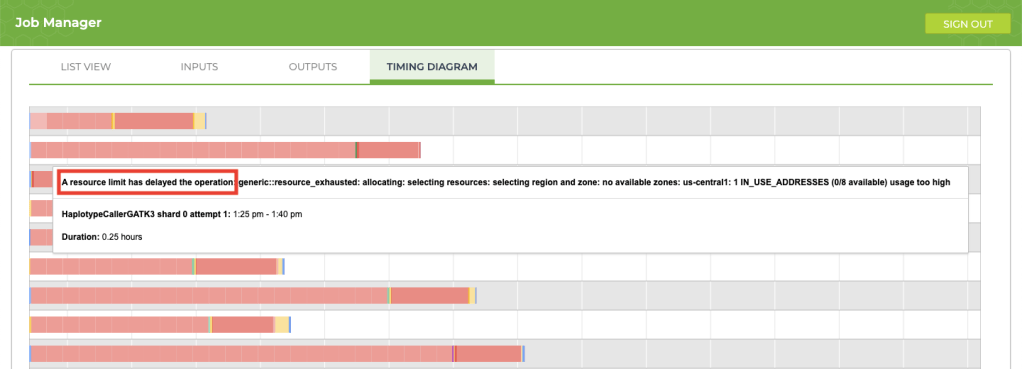
5. Improving process delays
If your job is taking longer than usual (say, an extra 12+ hours), take a look at the timing diagram in the Job Manager. If you see a bunch of pink boxes, it’s time to submit a request to Terra Support for more resources. To submit support requests, you must create a Zendesk account that is separate from your Terra account. The good news is that the support account that you create for Terra will also be valid for questions that you submit to the GATK Community Forum.
This article provides an excellent overview explaining how to request additional resources for your project. In my case, I wanted my jobs to run 30% faster, so I requested an increase for resources that were limited (IP addresses and CPUs). After forwarding my request, the support team took care of my request immediately and the issue completely disappeared. Here is the information that I provided for the request:
Your Terra billing project: YOUR-BILLING-PROJECT-GOES-HERE
Which quota(s) you want to increase: IP addresses and CPUs
What you want your new quota(s) to be: 30% higher than what they are now
Which regions you want the increase applied to, if applicable: us-central1
Rationale for increase: Research purposes
6. Information to include when submitting a support request
If you followed the instructions in the previous step, you are ready to submit support requests. Providing these items in your request will speed-up the process:
Your Project ID
Your workspace name
Your Bucket ID, Submission ID, and Workflow ID
Any useful log information
You may also be asked to share your workspace with the support team. To do this, add the email address GROUP_FireCloud-Support@firecloud.org to your workspace by clicking the Share button–the option is located in the three-dots menu at the top-right.
7. Cleaning up
My fifth run was successful! Now it was time to clean-up.
After learning how to use this workflow and running it unsuccessfully a few times, I had amassed a significant amount of storage. To wit:
$ gsutil du -s gs://my-terra-bucket-id
3,994,577,017,810  gs://my-terra-bucket-id
Holy smokes–about 4 terabytes, which costs more than $50 USD per month using standard Google cloud storage. At runtime, you can automatically delete intermediate files with an option that removes files for workflows that complete successfully. Since I was learning, I kept them around and then used the Remove_Workflow_Intermediates notebook to remove them manually.
To begin cleaning-up, I removed all subdirectories with failed runs (but not the notebooks directory):
The spinning circles show the directories that I manually deleted. Be sure to keep the “notebooks” directory.
Next, I looked at the size of the directory from my successful run, about 864 gigabytes:
$ gsutil du -s gs://my-terra-bucket-id/my-submission-id
863,761,741,217  gs://my-terra-bucket-id/my-submission-id
To manually delete the remaining intermediate files, I copied this notebook to my workspace. Note: Before running it, I upgraded to the latest version of pip and google-cloud-bigquery with this command:
Within the notebook code, I also modified the pip command to upgrade to the latest library versions with this command:
!pip install --upgrade $install_cmd
The program found 463 intermediate files to delete (Note: 782.61 GiB = 840 gigabytes).
WARNING: Delete 463 files totaling 782.61 GiB in gs://my-terra-bucket-id (Whole-Genome-Analysis-Pipeline)
Are you sure? [y/yes (default: no)]: yes
After executing the cleanup code, I reduced total storage for the successful run by 97%, from about 864 to 23 gigabytes, which now costs less than $0.50 USD per month using standard Google cloud storage. The largest savings came from storing the uncompressed BAM file (previously 80 gigabytes) as a compressed CRAM file (16 gigabytes). My take-home: It pays to pay attention to unnecessary files!
Conclusion
After building uBAM files correctly, reprocessing my genome would typically cost about $7 USD and three days of compute time. It took five runs to get it right, but Terra’s call caching magic–and perhaps the additional CPU power that I requested–brought the last runtime down to 14 hours. It has been a steep climb, but the views are great. Next up: reprocessing WGS data for the rest of our family, and then joint variant calling.
This entry was cross-posted from Terra on April 28, 2021.
In April, we celebrate Citizen Science Month, World Autism Day, and National DNA Day. In this guest blog post, all three events come together as KT Pickard, father of a young woman with autism, shares his family’s story of personal genomics and citizen science.
This past Sunday was National DNA Day, which commemorates the discovery of DNA’s double helix in 1953 and the publication of the first draft of the human genome in 2003. Events on National DNA Day celebrate the latest genomic research and explore how those advances might impact our lives. Last year, I wrote a playful article for DNA Day that investigated whether genetics is truly like finding a needle in a haystack. This year, our family is honored to share our story and ideas with you.
Our family’s DNA odyssey
My wife and I have a young adult-aged daughter who is on the autism spectrum. We first discovered that our daughter had autism when she was eight years old. As we struggled to understand autism and what it meant for our family, we learned that autism is uniquely expressed: Meeting one person with autism means that you have met one person with autism.
Long fascinated with genomics, my wife and I wondered how our DNA may have contributed to her condition, and we set out to learn all that we could. It was the beginnings of this diagnostic odyssey that gave expression to my second career as a citizen scientist. My professional background in supercomputing, software engineering, and medical imaging were a good start to apply scientific principles and gain insights.
We began our journey by talking with our family doctor, then my wife and I had our whole genomes sequenced through the Understand Your Genome project. Later, we crowdsourced the sequencing of her genome and began looking for genetic clues. By applying trio analysis to our family data, we discovered some preliminary findings: Our daughter has deletions in the NRXN1 gene and in a large region of chromosome 16, which have been found to be widely associated with developmental issues including autism. It looks like my wife and I have each contributed some variant alleles, but we are being careful about interpreting these findings because our WGS data and our daughter’s were processed through different pipelines, which could lead to inconsistent results.
Trio analysis of the NRXN1 locus shows a compound heterozygous deletion, with each parent possibly contributing one allele (visualization by VarSeq from Golden Helix).
To continue our journey, I want to reprocess our family’s WGS data with the latest GATK Best Practices, in the hope that this will give us a consistent baseline. I came across Terra through the book Genomics in the Cloud, which I picked up to help me learn more about GATK. I led an online book club in early 2021 based on the book, and subsequently moved our WGS data to the Terra platform. Now I am using the GATK Whole Genome Analysis Pipeline in Terra to reprocess our data. Working with Terra has been challenging, but highly satisfying because it provides access to industry standard genomics tools.
From personal genomics to citizen science
My family’s main goal with this project is to make meaningful discoveries about the genetic basis of our daughter’s autism. In 2015, genetics could explain the heritability of autism spectrum disorder in approximately 1 in 5 cases. Amazingly, that number has increased to 4 in 5 cases today.
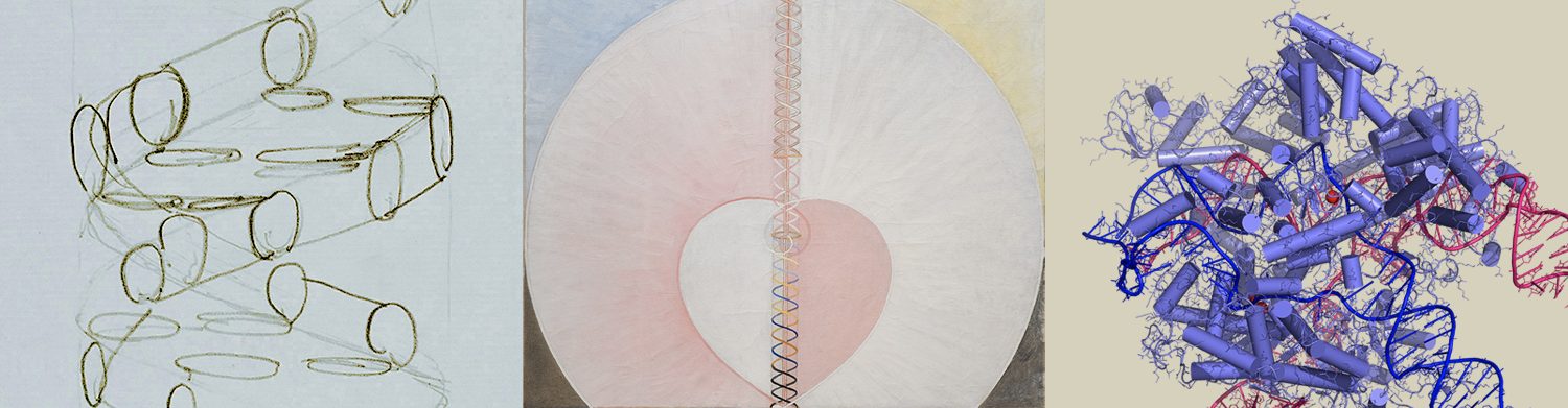
Our daughter (who drew this image) is on the left. At the time, she represented the 1 in 5 people whose autism could be explained by genetics.
Yet there is more to be gained. Although whole genome sequencing may not provide directly actionable results for autism itself, WGS can make a huge difference for parents who discover a comorbid, but treatable condition. By sharing our data and our findings with others, we can accelerate medical knowledge.
A growing number of projects offer opportunities for non-scientists to contribute in various forms to the advancement of biomedical research. In U.S. healthcare, one of the largest citizen science projects—All of Us—seeks one million people to share their unique health data to speed up medical research. By creating a national resource that reflects and supports the broad diversity of the U.S., the goal of All of Us is to advance precision medicine for all.
We have enrolled in the All of Us project and are looking forward to doing our part. I find it inspiring that this is something we can all contribute to, as citizens, even those of us who are not researchers.
Looking to the future
At its core, citizen science is a collaboration between scientists and those who are curious and motivated to contribute to scientific knowledge. As our family’s odyssey unfolds, I like to reflect about what I see out here on the bleeding edge of research, and how it could be applied to improve outcomes for patients in the real-world.
In community practice, many medical providers have limited knowledge of autism. Due to a lack of effective data sharing and awareness, an undiagnosed person with autism who walks through the door of a hospital may appear like a rare disease patient. A clinician evaluating them would miss out on a huge amount of valuable context. How could we improve the system so that clinicians could more effectively recognize the underlying context of that person’s condition? We can address some of these issues with machine learning, but that requires pooling together huge amounts of data, and much of that data is difficult to access.
As a citizen scientist, I see an enormous opportunity to combine research data with real-world data and evidence across healthcare delivery organizations. Common ontologies and interoperability standards are making it increasingly easy to pool de-identified datasets to test hypotheses on synthetic data—realistic-but-not-real data—to gain insights. A recent “call to action” encourages citizen scientists to evaluate the utility of this method precisely because data can be shared without disclosing the identities of anyone involved. Done ethically and responsibly, this synthetic DNA approach has the potential to accelerate autism research and deliver new benefits to patients.
This is the perspective I have gained from my journey so far. By asking questions and continuing to discover more about what our genomes contain, I have been fortunate to learn much about scientific principles, bioinformatics, and a bit about the genetic basis of autism. Although it is at times a challenging road, I have found that the path of personal genomics and citizen science is a satisfying way to find answers to the questions that my family faces. I hope this story will inspire others to explore, and perhaps let researchers and clinicians see patients and their families as potential collaborators in the quest to understand complex conditions like autism.
[Update: 2021-01-10: Thank you for your interest in our book club. We are currently closed to new members, but you can watch and subscribe to our meetings on the Genomics in the Cloud Book Club channel on YouTube.]
Introducing the Genomics in the CloudBook Club, an online discussion group. Our 35+ members across 10 time zones are covering one chapter each week, and we expect to complete the book in March 2021.
For a chapter synopsis, please read this Twitter thread from one of the authors, Geraldine A. Van der Auwera. My book review is available on Amazon.
Taking a page from the R for Data Science Online Learning Community, we created a Slack account for discussions and a Zoom account for meetings. Last week, we had lively online conversations about reference genome diversity, workflow language selection, personal whole genome sequencing, reproducibility tips, and more.
After each meeting, we post the video to this GITC Book Club channel on YouTube so you can follow us anytime. Our member’s tweets are also available here. Thank you for tuning in!
In this post, I explain how I created FASTQ files from a BAM file using a utility called Picard (no relation, although I pronounce my name the same way).
One of the limitations of the family trio work was that the bioinformatics pipelines were different between our samples and our kids’ samples. To fix this limitation, I had to “reconstitute” the original FASTQ files from the BAM file provided by Illumina and then re-run all our data through the same pipeline. (Note: To my knowledge, UYG no longer provides BAM files as part of this program.)
You can create FASTQ files from your BAM file by using Picard, a set of Java-based command line tools for manipulating high-throughput sequencing (HTS) data in formats such as SAM/BAM/CRAM and VCF.
Running Picard
For reasons that escape me now, I first ran Picard using an AWS t1.micro instance.
Facepalm: I attempted to run Picard using an AWS t1.micro instance. Source: Paramount
After 3 attempts–watching Picard fail after running for 3 days each time–and creating thousands of temp files in the process, I learned the hard way that Picard requires more than 613 MBytes of memory. This time, I used a c4.2xlarge instance (4 cores, 16 GBytes of memory), which worked. It appears that 16 GBytes is about the minimum amount of memory to get the job done.
Step 1. Is your BAM file sorted?
Before creating FASTQ files, make sure your BAM file is sorted so that your genome coordinates are in order. One of the ways to do this is with samtools, a suite of programs for interacting with HTS data. Here are the commands I used to install it. You can check whether or not your BAM file is sorted by using this command:
samtools stats YourFile.bam | grep "is sorted:"
# "is sorted: 1" = Yes, your BAM file is sorted.
# "is sorted: 0" = No, your BAM file is not sorted.
If your BAM file requires sorting, use this command (or something close to it):
# Type "samtools sort --help" for a description of this command
samtools sort -n -@ 2 -m 2560M InputFile.bam -o ./OutputFile.sorted.bam

# Check for existence of Read Groups (@RG)
samtools view -H InputFile.bam | grep '^@RG'
Step 2. Run Picard
Get Java and the picard.jar file. Run this command, but keep in mind that the options below are for a BAM file created on an Illumina HiSeq sequencer:
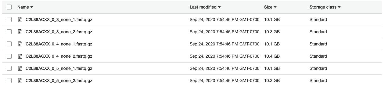
Using the c4.2xlarge instance, I ran Picard in 3 hours to create the FASTQ files shown below. In addition, creating compressed (gzip) versions of the files required another 8.5 hours of compute time. With an on-demand price of about $0.40 per hour, creating compressed FASTQ files cost approximately $4.60 USD on AWS.
In 2014, I uploaded my WGS data to the cloud and made it publicly available. In a previous post, I explained why I moved my WGS data from DNAnexus to Amazon. In this post, I explain the final step: attaching the S3 bucket to a web server. The goal was to replace the ftp server with a web server and make it easier to download my whole genome sequence data.
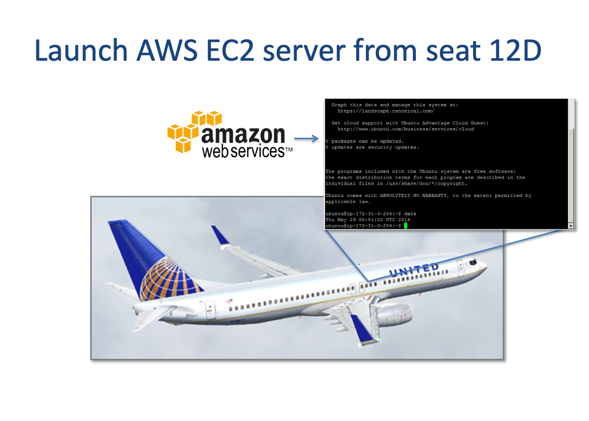
I launched my first cloud server literally while in the clouds in May 2014. Cloud computing has changed so much, it’s unbelievable. Back then, I had to patch the Linux kernel by hand so that the ftp server would work on AWS. Today, uploading your genome using Amazon’s command line interface (CLI) to an AWS S3 storage bucket is relatively easy. Understandably, Amazon makes it challenging (but doable) to make your storage publicly available. I used the Apache Web Server and s3fs to share this information.
My first cloud server
Step 1. Install Apache
Depending on your flavor of Linux, your commands may vary. I am using Ubuntu 18.04 LTS running on a t2.micro EC2 server. Here are the commands I used to install the Apache HTTP Server.
Step 2. Install s3fs
s3fs allows allows you to mount an S3 bucket via FUSE. s3fs preserves the native object format for files, allowing use of other tools like AWS CLI. Again, your commands may vary depending on your flavor of Linux. Here are the commands I used to install s3fs.
$1,500. That’s the amount of money I have spent over the past 5 years to store our family’s whole genome sequence (WGS) data. For $299 per person in 2020, I could sequence all of us again at 30x coverage, get the same data files, and spend less money. In 2015, I wrote about posting my WGS data to DNAnexus. Last month (July 2020), I moved all of our data to Amazon (AWS) S3 storage. In this post, I explain why.
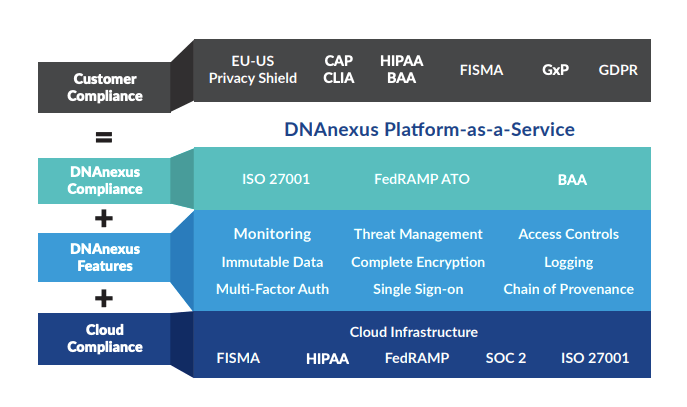
Five years ago, my impression was that DNAnexus was a platform for researchers, not consumers. It turns out that my first impression was correct–DNAnexus is not a platform for consumers. To their credit, their platform-as-a-service model includes an extensive set of genomic analysis tools, an easy-to-use SDK,top-notch documentation. a way to run your own docker images using Workflow Description Language (WDL), and a professional services team. DNAnexus’ IT infrastructure and regulatory compliance make the platform valuable for over 100 enterprise customers, and their recent $100M funding round coupled with their UK Biobank/AWS announcement will enable the company to expand into new markets and let researchers find more actionable insights.
DNAnexus Platform-as-a-Service
Nevertheless, I recently moved my WGS data to Amazon S3 due to storage costs and a lack of price transparency.
Storage costs
I’ve learned that most of the work that I want to do can be done with VCF files. Yes, there are times when I want to look at BAM files, but moving those files to lower-cost storage makes sense. DNAnexus introduced a Glacier-based archiving service in 2019 to support those operations, although I did not use it. My BAM file is 73 GBytes, which represents about 93% of the 79 GBytes for my WGS data (no FASTQ data). If I deeply archive BAM and FASTQ data (329 GBytes total), I can reduce the amount of higher-cost storage by 98%. The cost comparison for a single genome with FASTQ files looks roughly like this:
Storage cost on DNAnexus: (329 GBytes * $0.03 per GB-month [everything]) = $9.87 per month
Storage cost on AWS: (7 GBytes * $0.0125 per GB-month [VCF]) + (322 GBytes * $0.00099 per GB-month [everything else]) = $0.41 per month
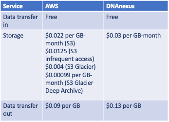
Overall, I can reduce my monthly storage costs by over 95% by using lower-cost storage tiers on AWS (see Table 1 below). Again, the comparison is apples-to-oranges because I did not use DNAnexus’ archiving service, mostly because it required a separate license to activate. Using Amazon S3, our monthly WGS storage costs will decrease from $24 per month to less than $1 per month.
Table 1. Comparison of AWS and DNAnexus storage pricing (accessed August 23, 2020).
Lack of price transparency
If we compare AWS’ S3 storage price from 5 years ago to DNAnexus’, we find that the storage markup was 35% over the S3 list price. It turns out that Amazon decreased its S3 storage price over the past 5 years, which led DNAnexus to drop their storage price to the current $0.03 per GB-month, still at a 35% markup. (For comparison, on demand GPU- or FPGA-based compute cycles (Amazon EC2) are marked-up over 100%.)
I do not fault DNAnexus for marking-up AWS pricing–they are a business and provide value beyond storage and compute cycles. However, you will not find any pricing information on the DNAnexus website. In addition to storage costs, add-ons like archiving and GxP regulatory compliance require separate licenses that are not disclosed when signing-up. Presumably, the company’s professional services team assists with these onboarding activities.
How to move your data from DNAnexus to AWS
So, having made the decision to move my WGS data to AWS, how did I do it?
On the DNAnexus platform, I used AWS S3 Exporter, a company-provided tool to upload data to an AWS S3 bucket (DNAnexus account required). You can invoke the exporter using either their SDK (dx-toolkit) or an online wizard–both methods work great. The DNAnexus policy documentation does not include verification by default, so I updated the AWS IAM policy file with a resource-based policy and also enabled transfers to work with verification:
Another improvement: You can transfer your data from one S3 instance to another (DNAnexus to AWS) at the rate of 250 GBytes per hour, including verification. Five years ago, the transfer speed was 10 GBytes per hour!
One final gotcha
One thing that has not changed in 5 years is the “data transfer out” fee. Amazon’s fee is $0.09 per GByte and DNAnexus’ fee is $0.13 per GByte. This fee is an understandable disincentive to keep you from moving your data around too much. In my case, moving our family’s WGS data to AWS will add over $100 to the final bill. It’s a little like losing all your money at baccarat and then finding out that you still owe the banque a commission before you leave the table. Not a big deal when you are a family, but when you are the UK Biobank expecting to grow to 15 petabytes over the next 5 years…well, you get the idea.
For the money, take a look at upstart competitors like Basepair or ixLayer.
[Update 2021-01-10: Do not forget to remove the DNAnexus API, called dx-toolkit!]
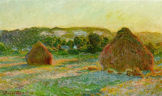
You may know this painting, one of over two dozen haystack paintings (actually, stacks of wheat) that Claude Monet produced at various times and seasons. What if we hid a needle one of them? Could we find it? In genetics, we often say that finding a genetic variant is like finding a needle in a haystack. But how big is the needle? How big is the haystack? Who believes this stuff?
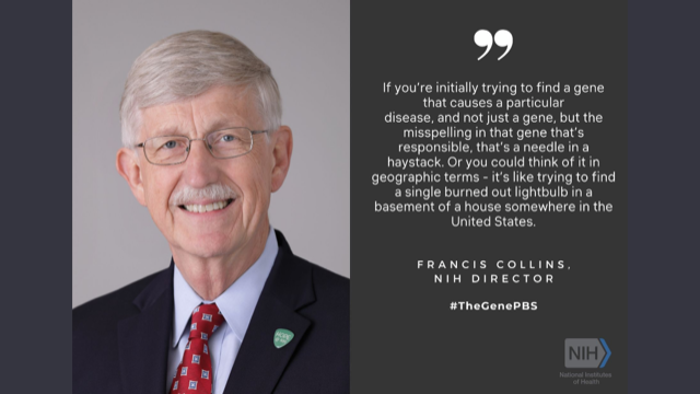
Francis Collins, NIH director and leader of the Human Genome Project, is a clear believer. In a recent PBS series by Ken Burns, The Gene: An Intimate History, Dr Collins said that finding a misspelling in a gene that causes a particular disease is “a needle in a haystack.“
Dr Francis Collins, NIH director
So, in honor of April 25th, National DNA Day, which commemorates the discovery of DNA’s double helix in 1953 and the publication of the first draft of the human genome in 2003, I embarked on a curious journey to answer these questions. My approach would be to determine the volume of a needle and then figure out how large to make the haystack to see if the analogy holds.
What is the volume of a needle?
How do you calculate the volume of a needle? It is useful to start with some real needles, and it turned out that I had a small box of 30 assorted needles–here’s a photo of them:
30 needles ranging is size from 30 mm to 60 mm
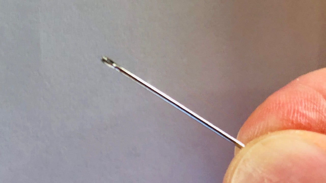
Needles come in all kinds of lengths, but I was looking for an “average” needle, so I made a rough list of their lengths and came up with this:
Average needle length: sum(5 x 30 mm, 10 x 35 mm, 11 x 40 mm, 1 x 45 mm, 1 x 50 mm, 1 x 55 mm, 1 x 60 mm) / 30 = 37 mm or 1.4 inches
A very average needle from my sample (length = 37mm, diameter = 0.75 mm)
Volume of a needle: displacement method
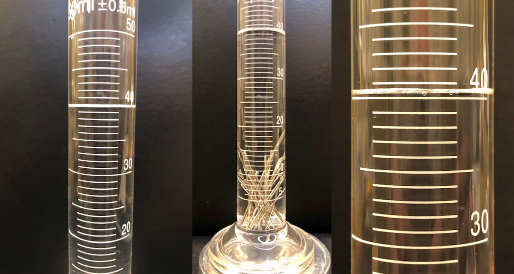
Next, I had to figure out the volume (V) of a needle. My first approach was to drop the needles into a graduated cylinder filled with water and then measure the displacement.
Graduated cylinder filled with 40 ml water (left). Needles in graduated cylinder (middle). Close-up photo showing 0.5 ml water displacement (right).
It turns out that 30 needles displaced 0.5 ml of water, so we divide by 30 to get the average volume of the needles in my sample.
V = 0.5 mm / 30 = 0.016 ml or about 0.02 ml per needle
Can we find a different method to measure the volume of the needle and compare results?
Volume of a needle: small cylinder
Another way to approximate the volume of the needle is to view it as a small cylinder using the formula: V = pi * r^2 * height. Since we are looking for volume (V), we want to express our measurements in centimeters to end up with cubic centimeters (cc).
V = pi * (0.075 cm / 2)^2 * 3.7 cm = 0.016 cc, or about 0.02 cc
Since 1 ml = 1 cc, we can say that the volume of our needle is 0.02 ml, which is spot on with our previous measurement. Note: It is rare in science that your numbers match exactly, but we’ll take the win and start building our haystack.
Building a genetic haystack
Our next task is to build a haystack that approximates the size of the human genome, where each A-T or C-G base pair in the human genome is the size of a needle. The Human Genome Project pegs that number around 3 billion base pairs within one copy of a single genome.
We build our genetic haystack by defining it as a volume having 3 billion opportunities to find a 0.02 ml object, or volume (V) equals 3,000,000,000 * 0.02 ml.
V = (3*10^9 * 0.02 ml) = 60*10^6 ml or 60,000,000 ml
Since 1 ml = 1 cubic centimeter (cc), the volume can also be stated as 60,000,000 cubic centimeters or 60*10^6 cc. Finally, 1 liter = 1000 ml, so the volume in liters equals 60,000,000 ml * (1 liter / 1000 ml).
V (haystack) = (60*10^6 ml) * (1 liter / 1000 ml) = 60*10^3 liters or 60,000 liters
We now know how much space it occupies, but what does it look like? For example, how tall is our haystack?
Shape of a genetic haystack: approximation with a hemisphere
Like the needle, we can approximate the shape of a haystack to something easy to calculate, like the volume of hemisphere in cubic centimeters: V = 2/3 * pi * r^3.
V (hemisphere) = 60*10^6 cc = 2/3 * pi * r^3
Solving for the radius (r), we get r = 306 cm. Since 1 m = 100 cm, the height (radius) of the hemisphere equals 306 cm * (1 m / 100 cm).
r (hemisphere) = 306 cm * (1 m / 100 cm) = about 3 meters or 10 feet tall
So, we have a rough idea of what an idealized haystack looks like. It is 3 meters tall and it is shaped like a hemisphere. But how accurate is our measurement? Can we do better? Has anyone studied haystack modeling? Indeed, someone has and his name is W.H. Hosterman.
Shape of a genetic haystack: using haystack modeling
Outline drawings of square hay stacks of different shapes
In 1931, W.H. Hosterman from the U.S. Department of Agriculture published an extensive technical bulletin “for the purpose of determining the volume and tonnage of hay.” Hosterman and his USDA colleagues measured over 2,600 haystacks across 10 states and presented results for both square and round haystacks. For round haystacks, Hosterman derived this formula: V = ((0.04 * Over) – (0.012 * C)) * C^2, where C is the circumference of the haystack, and Over is the measurement of the circumference of the stack over the top. We can compare results with the hemisphere by selecting equivalent values from Table 7 in Hosterman’s paper. (We will momentarily switch to imperial units to make use of the constants in the formula.)
The observed height of Hosterman’s haystacks are slightly taller than wide, but their sloped tops make the volume of the “true” haystack (58,333 liters) a little less than our original estimate of a 3-meter-tall, 60,000-liter haystack. When we compare the volume using Hosterman’s formula to the volume of the hemisphere, we see that they differ by 1,667 liters, or about 3%. Close enough!
Genetics is like finding a needle in a haystack
We have two comparisons that match closely. So, what does that haystack look like?
Romanian haystacks are typically 3 to 4 meters tall.
It turns out that Romanian haystacks are about 3 meters tall, so finding a misspelling in a gene (a genetic variant) is indeed like finding a needle in a haystack.
Who looks for needles in haystacks?
If genetics truly is like finding a needle in a haystack, what kinds of people do this? Well, let’s go back to Francis Collins.
In 1993, Collins published a paper describing the genetics of cystic fibrosis, a disease that required finding “a needle in a haystack.” Today, we have found needles from thousands of genetic haystacks. Some of these needles lead to clues about rare diseases, which affect more than 400 million people worldwide.
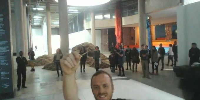
In real life, you can find a needle in a haystack, too. In 2004, performance artist Sven Sachsalber found a needle in a haystack after hunting for it for 24 hours. If we could get computers to solve diseases at that speed, we would happily be out of work.
In 2004, performance artist Sven Sachsalber found a needle in a haystack at the Palais de Tokyo in Paris.
Today I joined All of Us, a research community of one million people to lead the way for individualized prevention, treatment, and care for, well, all of us. This project was previously known as the Precision Medicine Initiative.
Many of you know that our family has used whole genome sequencing to look for clues in our daughter’s autism. This blog shares that journey. I have also published peer-reviewed papers to explore the reasons why people share personal health information. Through this research, I am convinced that information sharing will contribute to a learning healthcare system to improve care and lower costs.
It just takes people like you and me to #JoinAllofUs and lead by example.